Fastest network-SIR code in the East

Update May 12, 2020. I rewrote this code in Fortran.

Update July 30, 2018. I just realized that it is not needed to put the recovery events on the heap (stupid me). So I took some time to seriously squeeze out most from this approach. You can find the code at the Github page below. It’s 2-3 times faster now. An N = 10,000, m = 3, BA model network takes 0.35ms / outbreak for β = 0.3.

I needed some reasonably fast C code for SIR on networks. Funny enough, I just had C code for a discrete-time version, nothing for the standard continuous-time, exponentially-distributed duration of infection. Although there are book chapters written about this that are more readable than this post (and accompanied by Python code), I decided to write my own code from scratch* for fun. This post is about some of my minor discoveries during this coding and comments to the code itself (that you can get at Github . . it is reasonably well commented and well structured, I think, and should be instructive). Probably all points are discovered before (if not, it is anyway too little to write a paper about).

*Except some old I/O routines & data structures.

What I remember from Kiss et al. ’s book is that there are two different approaches: the Gillespie algorithm (1. Generate the time to the next event. 2. Decide what the next event will be. 3. Go to 1.) and event-driven simulation (1. Pick the next event from a priority queue. 2. Put future, consequential events in the queue. 3. Go to 1.). I decided to go for the latter, using a binary heap for the priority queue. The Gillespie algorithm comes with so much book-keeping overhead that I can’t imagine it being faster? (Or are there tricks that I can’t see?)

Using a binary heap to keep track of what the next event is turned out to be very neat. It is a binary tree of events (either a node getting infected or recovering) such that the event above (the “parent”) happens sooner than a given event, and the event below occurs later. As opposed to other partially ordered data structures, it fills index 1 to N in an array. Extracting and inserting events takes a logarithmic time of the size of the heap. There are two functions to restore the partial order of a heap when it has been manipulated—heapify-down for cases when a parent-event might happen later than its children, or heapify-up when a child event might happen sooner than its parent. Heapify-up is faster (briefly because one child has one parent, but one parent has two children). Anyways, here’s the pseudo-code for one outbreak (with a Python accent):

initialize all nodes to susceptible
get a random source node i
insert the infection event of i (at time zero) into the heap
 
while the heap is not empty:
             i := root of heap (the smallest element)
             if i is infected:
                         mark i as recovered
                         move the last element of the heap to the root
                         heapify-down from the root
             else: [1]
                         mark i infected
                         add an exponential random number to i’s event time
                         heapify-down from i
                         for susceptible neighbors j of i:
                                     get a candidate infection time t (exponentially distributed + current time)
                                     if t is earlier than i’s recovery time and j’s current infection time:
                                                 if j is not on the heap:
                                                             add it to the end of the heap
                                                 update the infection time and heapify-up from j [2]

Comments:
[1] i has to be susceptible here, it can’t be in the recovered state
[2] since this update can only make j’s next event time earlier, we can use heapify-up

I’m too lazy to make a full analysis of the running time. For an infection rate twice the recovery rate, it runs 3000 outbreaks / second on the (16000+ node) Brazilian prostitution data (the naïve projection of the original temporal network to a static graph) on my old iMac.

The greatest joy to code this is, of course, to conclude it matches theory. I will show tests for 10^7 averages of a graph that, although small, has a very complex behavior with respect to the SIR model and thus is a good test case.

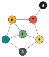
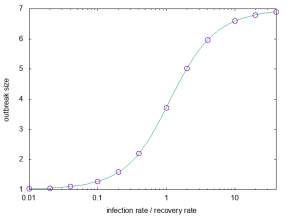
(In general, the most useful graphs for testing are complex enough for as many rare situations as possible to occur but small enough for signals from inconsistencies not to be drowned out by the rest of the network. Of course, you should (and I did) test different sizes.) For this graph, the expected outbreak size as a function of the infection rate x (assuming unity recovery rate) is exactly:

(1176*x^10+8540*x^9+26602*x^8+45169*x^7+46691*x^6+31573*x^5+14585*x^4+4637*x^3+977*x^2+123*x+7)/(168*x^10+1316*x^9+4578*x^8+9303*x^7+12215*x^6+10815*x^5+6531*x^4+2653*x^3+693*x^2+105*x+7)

The expression for the extinction time is much hairier:

(442496313262080000*x^40+27309066273423360000*x^39+807198400365952204800*x^38+15233070453900950384640*x^37+206427866398963479221760*x^36+2141932153788541338545664*x^35+17719320539717791500394656*x^34+120145769873280118142644464*x^33+681221206915024428485214000*x^32+3278911649316279397579655592*x^31+13554787582943216410512697434*x^30+48569821774947667173936604439*x^29+151963565615908045852605675638*x^28+417620288351605943926948229650*x^27+1012913280691378553984324143722*x^26+2176667408304962785107092061516*x^25+4157092031905378007476598228216*x^24+7073442188135283053895848231147*x^23+10743225033192917534525947880090*x^22+14584763731408596387436152087998*x^21+17714128509371287214419052953854*x^20+19257405578330410279734245444259*x^19+18738999678496655861828124214978*x^18+16315016288984176996492958607395*x^17+12698218026033692726424039694292*x^16+8823022276481055524449635661812*x^15+5462291880609485517543478166640*x^14+3005395264581878748317260429008*x^13+1464727118944592924512790487840*x^12+629657756169020017716116405376*x^11+237476658442269627398737860480*x^10+78048239230716482170978064640*x^9+22160762757395228067305587200*x^8+5376057161802601164632755200*x^7+1098215019757225723412736000*x^6+185258719580642643530649600*x^5+25115058278113706735616000*x^4+2629123086644412825600000*x^3+199399626889150464000000*x^2+9746072724455424000000*x+230390642442240000000)/(170659735142400000*x^40+10552460289638400000*x^39+312579991642963968000*x^38+5913391930417107763200*x^37+80362252019181365452800*x^36+836621475718722798182400*x^35+6948018151443087351091200*x^34+47327942978266352806656000*x^33+269810018795323799022182400*x^32+1307052538762076026520947200*x^31+5444452286343916086307449600*x^30+19683669375201197705776214400*x^29+62231912003456916355167472800*x^28+173109171912478541298715766400*x^27+425771864044847276704261819200*x^26+929669399656909987558520318400*x^25+1807917786488039546732408136000*x^24+3139331989062859723657121976000*x^23+4877014303846459457641565208000*x^22+6788014157540072132528114808000*x^21+8472216170656876854464167248000*x^20+9486363482241793767946469304000*x^19+9528536552497805862221968584000*x^18+8581068060934417967679452596800*x^17+6921355213421644368330335851200*x^16+4992142541382466682646297729600*x^15+3212789089879422999417773044800*x^14+1839664938944855009388405816000*x^13+933857320832833507287930597600*x^12+418340350779697721246663332800*x^11+164443976238518260207100150400*x^10+56319814910560911233147769600*x^9+16656366857169290147296243200*x^8+4205657447804826471220761600*x^7+893320008645089363572684800*x^6+156509988918986684124057600*x^5+22007772093708244924416000*x^4+2386316399921414553600000*x^3+187194956880347136000000*x^2+9449856184172544000000*x+230390642442240000000)

(How to calculate these expressions is the topic of this paper.) Anyway, they did immediately match perfectly (usually, plotting any consistency check like this sends me into another round of debugging):

  

All in all, it was a fun coding project (and quick—about 2 hr of primary coding and 3 hr of debugging . . no profiling or fine-tuning). Now let’s see if I can get some science done with it 😛

Without thinking too deeply, it might not be so straightforward to modify this code to the SIS model. It could be that one event changes many other events in the heap, which would make an event-based approach slow. In general, SIS is a much nastier model to study (computationally) than SIR. Both because it can virtually run forever, and that the fact that generations of the disease become mixed up prevents many simplifications (e.g., when calculating probabilities of infection trees).

Finally, the title of this post is, of course, a wink to FFTW (Fastest Fourier Transform in the West). I’m not sure this is the fastest code publicly available, but it shouldn’t be too far from it?