Crazy fast code for SIR on temporal networks

Now I turned this blog post into a paper.

This is a follow-up to my post a couple of days ago about all the nitty-gritty when coding up a compartmental model for empirical temporal networks. I guess the question lingering is: How do you do it then? There are a very straightforward way and an almost as simple, but much faster approach.

If you just want the code, get it here.

The simplest way of simulating the SIR model on a temporal network is to:

1. Mark all nodes as susceptible.
2. Run through the contacts.
3. Whenever a node gets infected (including the source), draws its time to recovery from an exponential distribution, and changes its state to I. Conveniently, one could represent the I state by the recovery time and let two out-of-bounds numbers represent S and R.
4. Stop the simulation when there are no infectious nodes.

There are a bunch of tricks one can do to speed up such a simulation. One can use bisection search to find the first contact capable of spreading the disease. One can calculate when nodes become inactive in the data and break the simulations when there are no active contacts left, etc. Still, this approach will be linear in the number of contacts C. Now consider the contacts between two nodes. Only one of these can transmit the disease. So clearly, if we can calculate which one that is and skip the other contacts, we will speed up the program a lot.

The slightly more complicated approach sometimes goes under the name event-driven simulation. It is conceptually so simple that I’m sure it has been invented and reinvented many times. (The idea comes from my static network code that was much inspired by Kiss, Miller & Simon’s book. I think I knew about the ideas already earlier, but I can’t remember from where . . at least the basic ideas are not my own.) The idea is:

1. Pick the next node i to be infected from a (priority) queue (ordered by the value of the nodes’ future infection times).
2. Draw the duration of i’s infection from an exponential distribution.
3. Calculate the future contacts with i’s neighbors that could spread the disease (maximum one per neighbor).
4. If such a future contact with a neighbor j happens earlier than the current infection time of j, then update the queue.
5. Go to 1 unless the queue is empty.

This turns out to be very efficient because:

• Steps 1 & 4 can be implemented efficiently. I use a binary heap where all operations are bounded by the logarithm of the size of the heap.
• Step 3 can also be implemented very fast. First, find the first contact between i and j after i becomes infectious. This can be done in logarithmic time (of the number of contacts between i and j) by bisection search. Then the process of transmitting the disease along the edge is effectively a sequence of Bernoulli trials with probability β. Thus the probability the k’th contact will be the one to transfer the disease is β (1 ­– β)^k–1. One can quickly draw a number (k) with this probability by

  floor [log (1 – X) / log (1 – β)]

  where X is a random variable in [0,1). If one gets a number larger than the number of remaining contacts, then i won’t infect j.

• Finally, by sorting the adjacency list (the list of a node’s neighbors) in decreasing order of their last contact, one only has to go through the active contacts at step 3 above.

In the worst case, this algorithm takes O(M + log C) time, where M is the number of edges (pairs of nodes with at least one contact). The speed-up is thus most substantial for data sets with many contacts per node (or edge).

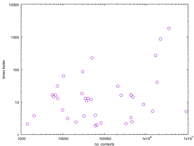
Below is a comparison between the two methods of all the 40-something data sets of this paper (β = 0.2 and ν = 5/T, where T is the duration of the data set). Large-C data sets have much time to be saved by using event-based modeling, but many higher-order effects make the speed gains differ from the worst case. It is worth noting that for none of the data sets, the reference algorithm is faster (even though in some extreme cases of low C vs. M that should be possible).

Finally, some of you might ask: what about the Gillespie algorithm? Somehow, the Gillespie algorithm has an undeservedly good reputation among my peers . . While the event-based method can be described as one think about the disease spreading processes, IMHO the Gillespie algorithm can’t. The step where one selects what to do usually comes with so much bookkeeping overhead that I have a hard time believing it would ever be fast. Two of my favorite network scientists Christian Vestergaard and Mathieu Génois (I’m pretty sure their work on randomization methods will be awarded the Temporal Network Paper of the Year 2018!), have a PLOS Comp. Biol. about the Gillespie algorithm for compartmental models on temporal networks. I played around with their code and . . long story short, I don’t think it is close to as fast as my code (I didn’t try all data sets or parameter values, so some disclaimer, but anyway). They have code for many versions of the SIR model, so it might be worth checking for that reason (but even for those cases, I think there are faster algorithms).

Absolutely finally, let me do an (anti) Fermat: A couple of summers ago, I was exploring fundamentally different temporal-network SIR algorithms that would exploit very different types of redundancies. I think I found a way to e.g., calculate outbreaks for all β values simultaneously (I just had some minor mysteries to solve). Still, it was quite convoluted, and it only took too long to fix the details (there is not enough space in this margin to explain the ideas!). So in the spirit of my motto: “it’s never too late to give up,” I gave up.