I do. In the sense of phantom traffic jams—traffic jams without a bottleneck, that just emerge spontaneously (and with peculiar density characteristics—more below). The most fundamental feature of highway traffic is the “inverse-λ shape” flow-density diagram. Flow is the number of vehicles that pass a point along the road. Density is how many cars there are per distance along the road.

At the left leg of the mirrored λ, cars can set their own pace, so the more cars, the higher flow. At the right leg, there is serious congestion all the way to complete standstill. In between these trivial phases, as often in complex systems, something interesting can happen—namely, phantom traffic jams.
I have no experience in traffic modeling and no ongoing projects about it but have been reading up on it for some related overview paper I’m writing. One thing that immediately strikes me, and probably any newbie to traffic modeling, is that basically all articles discussing phantom traffic jams—whether they are reviews or original research papers—illustrates it with the same figure:

The data came from aerial photography from Australia in 1967. It shows the trajectories of one lane of a highway (the truncated trajectories come from lane changes). It definitely feels weird that—if phantom traffic jams really are important—people don’t bother to use newer representative examples.
I decided to look for phantom traffic jams in the most extensive publicly available data set of car trajectories—the HighD data. This data set covers many car densities, but (unfortunately) most are in a free-flow state:
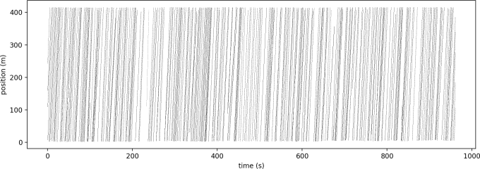
None of the 338 plots like this (showing the trajectories of traffic in one lane of multi-lane highways), is extremely congested. Some show stop-and-go waves:

But none shows as clear high-density waves as the Australia 1967 picture (that I take are characteristic of phantom jams—although I haven’t found a practical definition). Maybe this is the closest:

But these are waves primarily characterized by speed changes rather than an increased density.
Given that they have been spotted at least once and are predicted by traffic models that correctly describe most other aspects of highway traffic, I don’t doubt that phantom traffic jams exist. However, the outstanding questions for future research are: How common are they? Can models accurately reproduce their frequency?
The code for generating the figures is here. Thanks to Sun Lijun and Meead Saberi, who indirectly made me find the HighD data (by pointing me to the NGSIM data (that is hiding very well for being “publicly available”)).
